DARE TO COMPARE – PART 3

Parts 1 and 2 of Dare to Compare summarized fundamental topics about simple statistical comparisons. Part 3 shows how those concepts play a role in conducting statistical tests. The importance of these concept are highlighted in the following table.

Test Specification	Why it is Important
Population	Groups of individuals or items having some fundamental commonalities relative to the phenomenon being tested. Populations must be definable and readily reproducible so that results can be applied to other situations.
Number of populations being compared	The number of populations determines whether a comparison can be a relatively simple 1- or 2-population test or a complex ANOVA test.
Phenomena	The characteristic of the population being tested. It is usually measured as a continuous-scale attribute of a representative sample of the population.
Number of phenomenon	The number of phenomenon determines whether a comparison will be a relatively simple univariate test or a complex multivariate test.
Representative sample	A relatively small portion of all the possible measurements of the phenomenon on the population selected in such a way as to be a true depiction of the phenomenon.
Sample size	The number of observations of the phenomenon used to characterize the population. The sample size contributes to the determinations of the type of test to be used, the size of the difference that can be detected, the power of the test, and the meaningfulness of the results.
Hypotheses	You start statistical comparisons with a research hypothesis of what you expect to find about the phenomenon in the population. The research hypothesis is about the differences between the categories of the variable representing the population. You then create a null hypothesis that translates the research hypothesis into a mathematical statement that is the opposite of the research hypothesis, usually written in term of no change or no difference. This is the subject of the test. If you do not reject the null hypothesis, you adopt the alternative hypothesis.
Distribution	Statistical tests examine chance occurrences of measurements on a phenomenon. These extreme measurements occur in the tails of the frequency distribution. Parametric statistical tests assume that the measurements are Normally distributed. If the distribution is different from the tails of a Normal distribution, the results of the test may be in error.
Directionality	Null hypotheses can be non-directional or two-sided (i.e., ц=0), in which both tails of the distribution are assessed. They can also be nondirectional or one-sided (i.e., ц<0 or ц>0), in which only one tail of the distribution is assessed.
Assumptions	Statistical tests assume that the measurements of the phenomenon are independent (not correlated) and are representative of the population. They also assume that errors are normally distributed and the variances of populations are equal.
Type of test	Statistical tests can be based on a theoretical frequency distribution (parametric) or based on some imposed ordering (nonparametric). Parametric tests tend to be more powerful.
Test Parameters	Test parameters are the statistics used in the test. For t-tests using the Normal distribution, this involves the mean and the standard deviation. For F-tests in ANOVA, this involves the variance. For nonparametric tests, this usually involves the median and range.
Confidence	Confidence is 1 minus the false-positive error rate. The confidence is set by the person doing the test before testing as the maximum  false-positive error rate they will accept. Usually, an error rate of 0.05 (5%) is selected but sometimes 0.1 (10%) or 0.01 (1%) are used, corresponding to confidences of 95%, 90%, and 99%..
Power	Power is the ability of a test to avoid false-negative errors (1-β). Power is based on sample size, confidence, and population variance and is NOT set by  the person doing the test, but instead, calculated after a significant test result..
Degrees of Freedom	The number of values in the final calculation of a statistic that are free to vary. For a t-test, the degrees of freedom is equal to the number of samples minus 1.
Effect Size	The smallest difference the test could have detected. Effect size is influenced by the variance, the sample size, and the confidence. Effect size can be too small, leading to false negatives, or too large, leading to false positives.
Significance	Significance refers to the result of a statistical test in which the null hypothesis is rejected. Significance is expressed as a p-value.
Meaningfulness	Meaningfulness is assessed by considering the difference detected by the test to what magnitude of difference would be important in reality.

Normal Distributions

After defining the population, the phenomena, and the test hypotheses, you measure the phenomenon on an appropriate number of individuals in the population. These measurements need to be independent of each other and representative of the population. Then, you need to assess whether it’s safe to assume that the frequency distribution of the measurements is similar to a Normal distributed. If it is, a z-test or a t-test would be in order.

Yes, this is scary looking. It’s the equation for the Normal distribution. Relax, you will probably never have to use it.

This figure represents a Normal distribution. The area under the curve represents the total probability of measured values occurring, which is equal to 1.0. Values near the center of the distribution, near the mean, have a large probability of occurring while values near the tails (the extremes) of the distribution have a small probability of occurring.

In statistical testing, the Normal distribution is used to estimate the probability that the measurements of the phenomenon will fall within a particular range of values. To estimate the probability that a measurement will occur, you could use the values of the mean and the standard deviation in the formula for the Normal distribution. Actually though, you never have to do that because there are tables for the Normal distribution and the t-distribution. Even easier, the functions are available in many spreadsheet applications, like Microsoft Excel.

Statistical tests focus on the tails of the distribution where the probabilities are the smallest. It doesn’t matter much if the measurements of the phenomenon follow a normal distribution near the mean so long as it does in the tails. The z-distribution can be used if the sample size is large; some say as few as 30 measurements and others recommend more, perhaps 100 measurements. The t-distribution compensates for small sample sizes by having more area in the tails. It can be used instead of the z-distribution with any number of samples.

The concept behind statistical testing is to determine how likely it is that a difference in two populations parameters like the means (or a population parameter and a constant) could have occurred by chance. If the probability of the difference occurring is large enough to occur in the tails of the distribution, there is only a small probability that the difference could have occurred by chance. Differences having a probability of occurrence less then a pre-specified value (α) are said to be significant differences. The pre-specified value, which is the acceptable false positive error rate, α, may be any small percentage but is usually taken as five-in-a-hundred (0.05), one-in-a-hundred (0.01), or ten-in-a-hundred (0.10).

Here are a few examples of what the process of statistical testing looks like for comparing a population mean to a constant.

One Population z-Test or t-Test

All z-tests and t-tests involve either one or two populations and only one phenomenon. The population is represented by the nominal-scale, independent variable. The measurement of the phenomenon is the dependent variable, which can be measured using a nominal, ordinal, interval, or ratio scale.

For a one-population test, you would be comparing the average (or other parameter) of the measurements in the population to a constant. You do this using the formula for a one-population t-test value (or a z-test value) to calculate the t value for the test.

The Normal distribution and the t-distribution are symmetrical so it doesn’t matter if the numerator of the equation is positive or negative.

Then compare that value to a table of values for the t-distribution (for the appropriate number of tails, the confidence (1- α), and the degrees of freedom (the number of samples of the population minus 1). If the calculated t value is larger than the table t value, the test is SIGNIFICANT, meaning that the mean and the constant are statistically different. If the table t value is larger than the calculated t value, the test is NOT SIGNIFICANT, meaning that the mean and the constant are statistically the same.

Example

Imagine you are comparing the average height of male, high school freshmen, in Minneapolis school district #1. You want to know how their average height compares to the height of 9th to 11th century Vikings (their mascot), for the school newspaper. Turn-of-the-century Vikings were typically about 5’9” or 69 inches (172 cm) tall.

This comparison doesn’t need to be too rigorous. The only possible negative consequence to the test is it being reported by Fox News as a liberal conspiracy, and they do that to everything anyway. You’ll accept a false positive rate (i.e., 1-confidence, α) of 0.10.

Nondirectional Tests

Say you don’t know many freshmen boys but you don’t think they are as tall as Vikings. You certainly don’t think of them as rampaging Vikings. They’re younger so maybe they’re shorter. Then again, they’ve grown up having better diets and medical care so maybe they’re taller. Therefore, your research hypothesis is that Freshmen are not likely to be the same height as Vikings. The null hypothesis you want to test is:

Height of Freshmen = Height of Vikings

which is a nondirectional test. If you reject the null hypothesis, the alternative hypothesis:

Height of Freshmen ≠ Height of Vikings

is probably true of the Freshmen. Say you then measure the heights of 10 freshmen and you get:

63.2, 63.8, 72.8, 56.9, 75.2, 70.8, 68.0, 64.0, 61.4, 65.2

The measurements average 66 inches with a standard deviation of 5.3 inches. The t-value would be equal to:

(Freshmen height – Viking height) / ((standard deviation / (√number of samples)))

t-value = (66 inches – 69 inches) / (5.3 inches / (√10 samples))

t-value = -1.790

Ignore the negative sign; it won’t matter.

In this comparison, the calculated t-value (1.79) is less than the table t-value (t_{(2-tailed, 90% confidence, 9 degrees of freedom)} = 1.833) so the comparison is not significant. The comparison might look something like this:

There is no statistical difference in the average heights of Freshmen and Vikings. Both are around 5’6” to 5’9” tall. That isn’t to say that there weren’t 6’0” Vikings, or Freshmen, but as a group, the Freshmen are about the same height as a band of berserkers. I’m sure that there are high school principals who will agree with this.

When you get a nonsignificant test, it’s a good practice to conduct a power analysis to determine what protection you had against false negatives. For a t-test, this involves rearranging the t-test formula to solve for t_beta:

t_beta = (sqrt(n)/sd) * difference – t_alpha

The t_alpha is for the confidence you selected, in this case 90%. Then you look up the t-value you calculated to find the probability for beta. It’s a cumbersome but not difficult procedure. In this example, the calculated t_beta would have been 1.24 so the power would have been 88%. That’s not bad. Anything over 80% is usually considered acceptable.

Most statistical software will do this calculation for you. You can increase power by increasing the sample size or the acceptable Type 1 error rate (decrease the confidence) before conducting the test.

So if everything were the same (i.e., mean of students = 66 inches, standard deviation = 5.3 inches) except that you had collected 30 samples instead of 10 samples:

t-value = (69 inches – 66 inches) / (5.3 inches / (√30 samples))

t-value = 3.10

t_{(2-tailed, 90% confidence, 29 degrees of freedom)} = 1.699

If you had collected 100 samples:

t-value = (69 inches – 66 inches) / (5.3 inches / (√100 samples))

t-value = 5.66

t_{(2-tailed, 90% confidence, 99 degrees of freedom)} = 1.660

These comparisons are both significant, and might look something like this:

More samples give you better resolution.

Directional Tests

Now say, in a different reality, you know that many of those freshmen boys grew up on farms and they’re pretty buff. You even think that they might just be taller than the Vikings of a millennia ago. Therefore, your research hypothesis is that Freshmen are likely to be taller than the warfaring Vikings. The null hypothesis you want to test is:

Height of Freshmen ≤ Height of Vikings

which is a directional test. If you reject the null hypothesis, the alternative hypothesis:

Height of Freshmen >Height of Vikings

is probably true of the Freshmen. Then you measure the heights of 10 freshmen and get:

72.4, 71.1, 75.4, 69.0, 75.7, 73.3, 76.0, 58.8, 70.4, 78.6

The measurements average 71.2 inches with a standard deviation of 5.3 inches. The t-value would be equal to:

(Freshmen height – Viking height) / (standard deviation / (√number of samples))

t-value = (72 inches – 69 inches) / (5.3 inches / (√10 samples))

t-value = 1.790

In this comparison, the table t-value you would use is for a one-tailed (directional) test at 90% confidence for 10 samples, t_{(1-tailed, α = 0.1, 9 degrees of freedom)} = 1.383. For comparison, the value of t_{(2-tailed, 0.9 confidence, 9 degrees of freedom)}, which was used in the first example, is equal to 1.833, as is t_{(1-tailed, 0.95 confidence, 9 degrees of freedom)}. The reason is that you only have to look in half of the t-distribution area in a one-tailed test compared to a two-tailed test. That means that if you use a directional test you can have a smaller false positive rate.

The table t value you would use, t_{(1-tailed, 0.1 confidence, 9 degrees of freedom)}, is equal to 1.383. which is smaller than the calculated t-value, 1.790, so the comparison is significant. The comparison might look something like this:

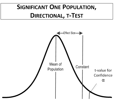
In this comparison, the Freshmen are on average at least 3 inches taller than their frenzied Viking ancestors. Genetics, better diet, and healthy living win out.

But what if the farm boys averaged only 71 inches:

 (Freshmen height – Viking height) / (standard deviation / (√number of samples))

t-value = (71 inches – 69 inches) / (5.3 inches / (√10 samples))

t-value = 1.193

The table t value you would use, t_{(1-tailed, 0.1 confidence, 9 degrees of freedom)}, is equal to 1.383. which is larger than the calculated t-value, 1.193, so the comparison is not significant. The comparison might look something like this:

And that’s what one-population t-tests look like. Now for some two-population tests in Dare to Compare – Part 4.

Read more about using statistics at the Stats with Cats blog. Join other fans at the Stats with Cats Facebook group and the Stats with Cats Facebook page. Order Stats with Cats: The Domesticated Guide to Statistics, Models, Graphs, and Other Breeds of Data analysis at amazon.com, barnesandnoble.com, or other online booksellers.